- >> Computing with spiking neurons
Computing with spiking neurons
Under construction !!!
Introduction
This practice aims at using spiking neurons to perform some computation. The spiking neuron models produce spike trains which are exchanged between neurons and we shall see in this practice that using appropriate connections between neurons, we can actually compute interesting things.
The simulations will be done with the Brian python simulator.
There is an appendix at the really end of this page where various python/brian pieces might be useful for writing the simulations.
Problem statement
We would like to build a spiking neural network able to recognize spatio-temporal sequences. For example, speech recognition, as introduced in a challenge by J.J. Hopfield and C.D. Brody in 2000 is one such sequences. They proposed in a paper entitled “What is a moment ? Cortical sensory integration over a brief interval”, simulated recordings of an artificial animal recognizing speech signals. They provided no indication on the model structure which allowed to generate these signals and proposed, in the challenge, to actually build up a spiking neuron model able to produce these signals.
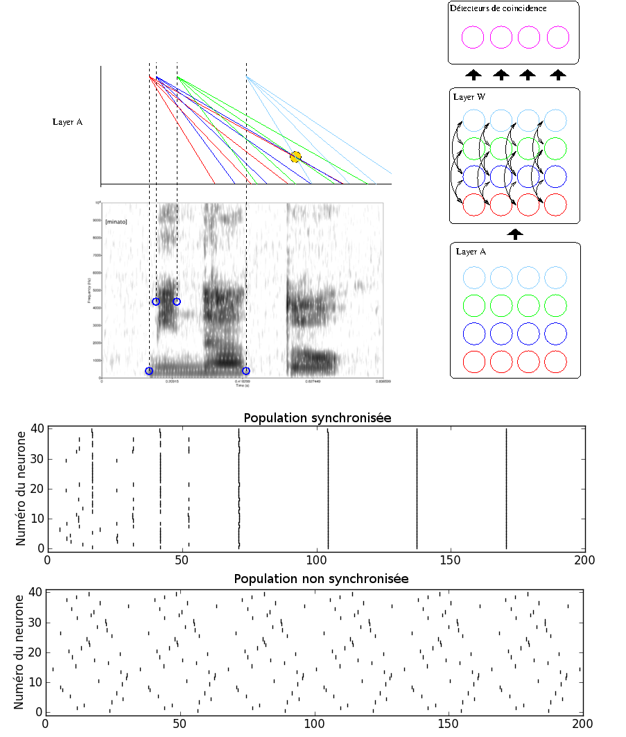
The model is built up of 3 layers. The layer A is filled with neurons detecting particular events of a spectrogram, like the appearance of a response in a given frequency band. In response to these particular events, several neurons will emit spikes at decreasing frequencies, starting when the event these neurons are selective to is detected. For a sequence of specific events, it happens that several neurons of the A layer have similar discharge frequency (which is indicated on the figure above by the yellow circle). As we will see, neurons might discharge with a similar frequency but with offsets in time. If we can make them trigger their spike at the same time, it is easier to detect the conjunction of events. Therefore, in the W layer, the neurons are coupled and this coupling will bring the neurons discharging in phase. We can then add, in a last layer, coincidence detectors which are just sensitive to, say, N neurons firing in a tiny time window.
We will build up the network step by step to get a glimpse on how sequence recognition might be implemented with spiking neurons. We will go through the following steps:
- observe that the discharge frequency of a leaky integrator neuron (one of the spiking neuron models) depends on the injected current
- observe that a population of spiking neurons, loosely coupled and discharging at a similar frequency discharge, get transiently synchronized
- detecting the coincidence of several spikes in a small time window (the transient synchrony above)
Taking a grip on Brian
Installing Brian
To install and keeping up to date python packages, we can use dedicated scripts: easy_install or pip. pip is somehow a better option as it allows to uninstall packages. Unfortunately, it is not necessarily installed by default. So we may use easy_install to install pip and then pip to install the other packages we need for the practice.
bash:user$ easy_install --user pip
The –user option ensures that the files are installed on your account, where you are allowed to copy files and more precisely, the packages are installed in “~/.local”.
You then have to set up some environment variables PATH and PYTHONPATH to find the pip binary and to inform python where to find packages installed with pip.
bash:user$ emacs ~/.basrc
>> export PYTHONPATH=$PYTHONPATH:~/.local/lib/python2.7/site-packages:~/.local/lib64/python2.7/site-packages
>> export PATH=$PATH:~/.local/bin/
You can then apply the changes by opening a new terminal or by simply calling the bash command source on ~/.basrc. We can now install Brian and its dependencies.
pip install --user matplotlib sympy brian
To test if you installation and setup were successful, launch a python console and try to import brian
bash:user$ python
Python 2.7.3 (default, Jul 24 2012, 11:41:34)
[GCC 4.6.3 20120306 (Red Hat 4.6.3-2)] on linux2
Type "help", "copyright", "credits" or "license" for more information.
>>> from brian import *
>>>
My first steps with brian
Brian is a python library. Python is a scripting language that you can learn quite quickly (you can do complicated things with Python but we will only use basic things here) and for which several libraries have been developed; for example Numpy for numerical computing, matplotlib to plot data, PIL to process images, sympy to perform symbolic computations, ...
If we have a look to a Brian script, we will find commands for:
- importing the brian library
- defining the parameters and equations of the model
- creating neural populations (with the NeuronGroup object)
- wiring neurons together (with the Connection and Synapses objects)
- specifying what to record during the simulation (with the SpikeMonitor and StateMonitor objects)
- launching the simulation (with a call to the run command)
- visualizing/analyzing the results
One can also run Brian in an interactive way but this is not what we going to do here. A basic brian script looks like below:
# -*- coding: utf-8 -*-

from brian import *

tau =   20 * msecond        # constant de temps
Vt =   -55 * mvolt          # seuil pour spiker
Vr =   -75 * mvolt          # potentiel de reset
Vs =   -65 * mvolt          # potentiel de repos
I0 =    15 * mvolt          # courant injecté
tmax = 500 * msecond        # durée de la simulation

# Notre groupe contient un neurone intègre et tire
eqs = '''
dV/dt = (-(V-Vs) + I)/tau : volt
I : volt
'''

G = NeuronGroup(N=1, model=eqs, threshold='V >= Vt', reset='V = Vr')

# On monitore ses spikes et son potentiel
spikemon = SpikeMonitor(G)
statemon = StateMonitor(G, 'V', record=0)

# On initialise le potentiel aléatoirement entre le reset et le seuil
G.V = Vr + (Vt - Vr) * rand(len(G))
G.I = I0

# On lance la simulation
run(tmax)

# On affiche combien de spikes ont été émis
print "Nombre de spikes émis : ", spikemon.nspikes

print "Liste des temps de spikes :"
print ', '.join(["%.3f ms" % (ts*10**3) for ts in spikemon[0]])
print "Temps inter-spikes (s.):\n",
print ', '.join(["%.3f ms" % ((t1-t0)*10**3) for t0, t1 in zip(spikemon[0][:-1], spikemon[0][1:])])

# On trace nos mesures
figure()
subplot(211)
for i, ts in spikemon.spikes:
    plot([ts/msecond, ts/msecond], [i, i+1], 'k')
ylim([-1,2])
xlim([0, tmax/msecond])
xlabel("Temps (ms)")
ylabel(u"Numéro du neurone")

subplot(212)
statemon.plot()
xlim([0, tmax/second])
ylabel('Potentiel (V)')
xlabel('Temps(s.)')

show()