- >> Softwares
- >> Singular Value Decompostion
Singular Value Decompostion
On this page, you will find some demos illustrating the use of Singular Value Decomposition. In the first example, the SVD is used to compress an image, while the second illustrates its use in optimizing the computation of convolution products.
An introduction on Singular Value Decomposition can be found in the wikipedia article on the SVD. More technical informations on how to actually compute this transformation can be found in Numerical Recipes, 3rd edition.
For the following, we just keep in mind that if \(M\) is a m-by-n matrix (real or complex), there exists a matrix \(U\), a diagonal matrix \(S\) n-by-n (with only positive or zero elements) and a n-by-b matrix \(V\) such that : \(M = U S V^T\) where \(.^T\) is the transpose operation. This transformation always exist and is based on applying the spectral theorem on the matrix \(M M^T\).
Image compression with Singular Value Decomposition
In this paragraph, you will find an example of image compression using the SVD. As we said above, the matrix \(\Sigma\) is a diagonal matrix. It contains the singular values of the matrix M that are, in the case of real matrices, positive. When you compute the SVD with standard tools (for example with the Gnu Scientific Library, or Scipy, but see the wikipedia page about the SVD for more references), the singular values are ordered in decreasing magnitude. To get successive approximations of the original image, we simply use more and more singular values (by decreasing magnitude) of the S matrix, by setting the others to zero.
Below is an example of image compression, done with the following script : svd_compress_image.py and the glade file svd_compress_image.glade. The example is written in Python, and requires in addition Matplotlib , numpy (for computing the svd) and PyGtk (for the bindings between Python and GTK).
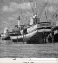
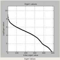
On the example below, the image size was 512x512 and the compressed image uses only 20 non-null eigen values, which means only 2 x 20 x 512 + 20 = 40 x 512 + 20 pixel values out of the 512x512 (2 sets of 20 vectors of the matrices U,V and 20 eigen values). The example below is in black and white but the script works also with color images.
| original image | Compressed image | Eigen values distribution |
|---|---|---|
 |
 |
 |
Convolution product with the Singular Value Decomposition
Interestingly, the SVD also allows to speed up convolution products. Basically, for some kernels, like gaussian kernels, the convolution is said to be separable in the sense that you can replace a 2D convolution by 2 1D convolutions. This can be seen from the SVD of the gaussian kernel which has a single non zero singular value.
The following script illustrates how to perform a convolution of a 2D-image with a gaussian kernel, using the SVD : svd_convolution.py . The script also contains additional code to load/save images and to evaluate the execution time. It requires Python, numpy and PIL .