Monte carlo swarm policy search¶

Inverted pendulum¶

The scripts for this simulation is available as CartPole.tar.gz.

In the inverted pendulum problem, we seek to determine the strength of a force applied to a cart on which a pendulum is anchored in order to maintain the pendulum still in the vertical position. The state space is defined with the angular position and angular velocity of the pendulum. The controller we seek to optimize involves 3 actions with one RBF network per action, each RBF network being made of 9 gaussians in the (theta,dtheta) space plus one constant term (the parameters are allowed to vary in the range [-100;100]). For each of the three actions (corresponding to forces of strength -50 , 0 and +50), the centers of the 9 gaussians are on [-\(\pi\)/4; 0 ; \(\pi\)/4] x [-1 ; 0 ; 1] . A probabilist toss is then used to select the action based on the probabilities of selecting each action as defined by their respective RBF network.

A random noise of +/- 5 N is added to the strength applied on the cart.

An episode starts with a pendulum randomy initialized in [-0.1 ; 0.1] x [-0.1;0.1]. It lasts at most 3000 iterations with a timestep of 0.1 s. If the pendulum reaches the horizontal position, the episode ends with a reward of -1, otherwise a reward of 0 is given at each interaction.

A particle of PSO hosts a set of parameters (in dimension \([-100;100]^{30}\)). The fitness of a particle is evaluated using several independent episodes. For the inverted pendulum, we used a single episode for evaluating the fitness during the iteration of the swarm and 500 episodes to get a better estimate of it for our own recording of the performance of the best controller found by the swarm. If a trial i lasted Ni steps, the fitness of the particle with P independent runs is the mean of -1/Ni . We seek to maximize this mean.

On the figure below, we show the mean length of an episode for the best particle of the swarm function of the number of swarm evaluations. The maximal lenght being 3000, the length of the episode.

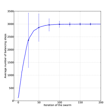
On the figure below, we show for different initial conditions, the number of balancing steps of the best controller as the swarm goes on. Suddenly, around 28 epochs, the controller performs perfectly from all the initial conditions.

Below we show two controllers trying to balance the pendulum starting at three different initial positions with a null speed. The first row is the initial best controller, the second one is the best controller found after few iterations. This second controller is able to avoid the pendulum from falling.

Controller #	\(\theta_0 = -0.1\)	\(\theta_0 = 0\)	\(\theta_0 = 0.1\)
Initial
Final

Mountain car¶

The scripts for this simulation is available as MountainCar.tar.gz.

In the mountain car problem we seek a controller able to drive a car out from a valley. The car is not powerfull enough to escape from it just keeping on accelarating. It has to go back and forth in the valley in order to get enough speed to exit.

The controller involves 30 parameters. We still have 3 actions and 10 parameters per action. The 10 parameters are a constant term plus the amplitude of 9 gaussians for a RBF network. The center of the gaussians are evenly spread in [-1.2,0.5]x[-0.07;0.07], these being the bounds for the horizontal position and velocity. The RBF networks give (unscaled) probabilities to select each actions. These values are scaled and used as probabilities for a random toss of the action.

Below, we show two controllers : an initial bad controller and the best controller the swarm has found. We started the car in the worst case. It takes 255 iterations for the first controller to exit the valley and only 115 for the best one.

Initial controller	Optimal controller

If we plot the number of steps it takes for the car to exit the valley function of the starting state (position and velocity), we obtain the figures below for the initial controller and the best controller found.

Initial controller	Optimal controller

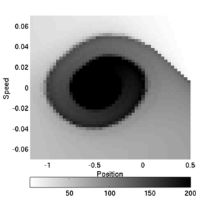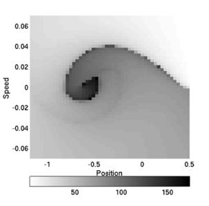Acrobat: underactuated double arm pendulum¶

The scripts for this simulation is available as Acrobat.tar.gz.

In the acrobot problem, we seek to optimize a controller for an underactuated double arm pendulum. The pendulum is starting at the vertical position, pointing down and we want to make it reach the vertical pointing-up unstable position.

Here we combine two controllers : a pre-computed Linear Quadratic Regulator and a RBF controller.

The LQR is computed with the following matlab scripts : jacobian_acrobot.m and lqr_acrobot.m. It is a linear controller with parameters K = [-240.7946 , -59.8844 , -88.3753 , -25.8847] (for the particular parameters of the system and time step we used). The strength given by this controller is computed as \(- K . [\theta_1-\pi/2; \theta_2 ; \dot{\theta_1} ; \dot{\theta_2}]\).

The RBF controller involves a RBF with \(4^4\) = 256 amplitudes of gaussians. We use 4 gaussians per dimensions and the state space has 4 parameters (two angular positions, two angular velocities). The strength given by this controller is a tanh of the result of the RBF, scaled by a maximal torque set to 2 Nm.

The control of the pendulum is switched from the RBF to the LQR as soon as the state [theta1;theta2;dtheta1;dtheta2] is in \([\pi/2 \pm \pi/4 ; 0 \pm \pi/2 ; 0 \pm \pi/4 ; 0 \pm \pi/2]\). This domain is quite large for the LQR; the LQR would not be able to maintain the pendulum is this whole subspace but the speed given by the RBF brings the pendulum in a narrower subspace where the LQR effectively stabilizes the pendulum.

Below we show two controllers. The first one is an inefficient controller which hardly brings the pendulum to the vertical position while the second one is one of the best controllers obtained after 4000 iterations of the swarm. On the illustrations, the second arm is plotted in green when a reward is a given.

Inefficient	Efficient