- >> Simulations
- >> Influence of spatial attention on the receptive field shape of neurons in monkey area MT
Influence of spatial attention on the receptive field shape of neurons in monkey area MT
Scripts
The Matlab scripts used for the theoretical curves of the paper are available here : attention_mt_scripts.zip. DivisiveInhibition.m is the script used for the 1D illustration, while Anton2D.m is the script used to generate the 2D illustration with the two antipreferred stimuli.
Exemple of receptive field modification
In experiments carried out in the group of S. Treue, a modification of the shape of monkey area MT neurons is observed when attention is inside versus outside of the receptive field. What is observed is a shift and expansion/shrinkage of the receptive field. We show below some examples of recorded receptive fields (for the experimental setup, please refer to the papers of the S. Treue group, co-authored with T. Womelsdorf and K. Anton-Erxleben) that have been fitted with splines.
| Attention outside | Attention inside | Difference in - out |
|---|---|---|
 |
 |
 |
Model
On several recordings, we observe both an increase of the receptive field on the side of the attentional focus and a decrease of the opposite flank of the receptive field. We proposed a divisive inhibition model that can account for these effects. The basic principle is very similar to the biased competition principle: spatial attention increases the effect of the stimuli below it. In the experiments we try to model, the stimuli behind the locus of attention are anti-preferred stimuli. We suppose that attending to these anti-preferred stimuli lead to an increase of inhibition of the recorded cell. However, the receptive field is mapped by flashing some preferred probes. In case a probe is flashed below the locus of attention, this will produce an increase of the response. The attention gated excitation/inhibition can lead to the observed modification of the receptive field. One model (but we can consider variations of it) we proposed is the following, that we state as a dynamic system that will be reduced to a steady state model. We model the response of the neuron to a probe flashed at position \(x\) as:
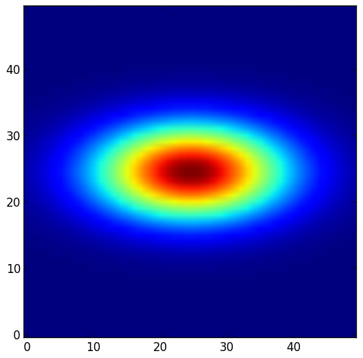
where \(x_{s1}, x_{s2}\) are the positions of the two anti-preferred stimuli S1 and S2 (see the description of the setup in the Womelsdorf et al. paper). \(r_{att}\) is the locus of attention taken as a gaussian centered on the attended point (which is enforced by the setup to be one of the two antipreferred stimuli lying inside the RF S1 or S2, or a stimulus in the opposite hemifield), \(g(x,t)\) is the unmodulated response taken as an elliptical gaussian to account for the orientation and variances of the RF. The equation above simply states that the neuron is excited by the probe by an amount depending on the location of the probe with respect to the RF center of the neuron and that the anti-preferred stimuli inhibit the neuron with a constant amount as these stimuli don’t move. Spatial attention is used as a booster of the excitatory/inhibitory influences of the various stimuli depending on their position with respect to the locus of attention.
If we look for the steady state reponses of the model above, we finally get a divisive inhibition model:
In the above equations \(r_away(x)\) is the response of the neuron to a probe flashed at position x, when attention is sufficiently far away from both the probe and stimuli S1 S2 to have no influence on them, it is an approximation of the more general \(r_{in}(x)\) response which can be used in all the situations.
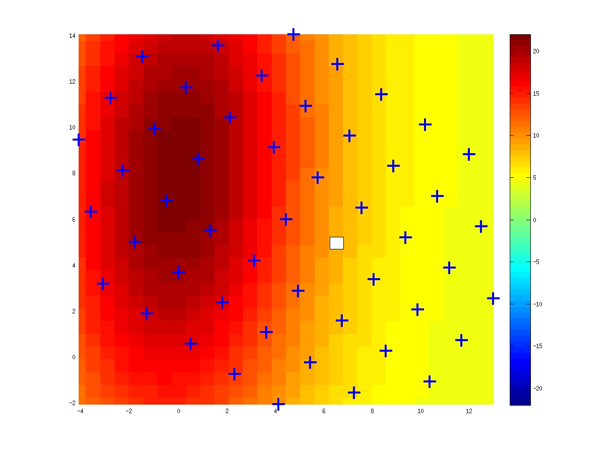
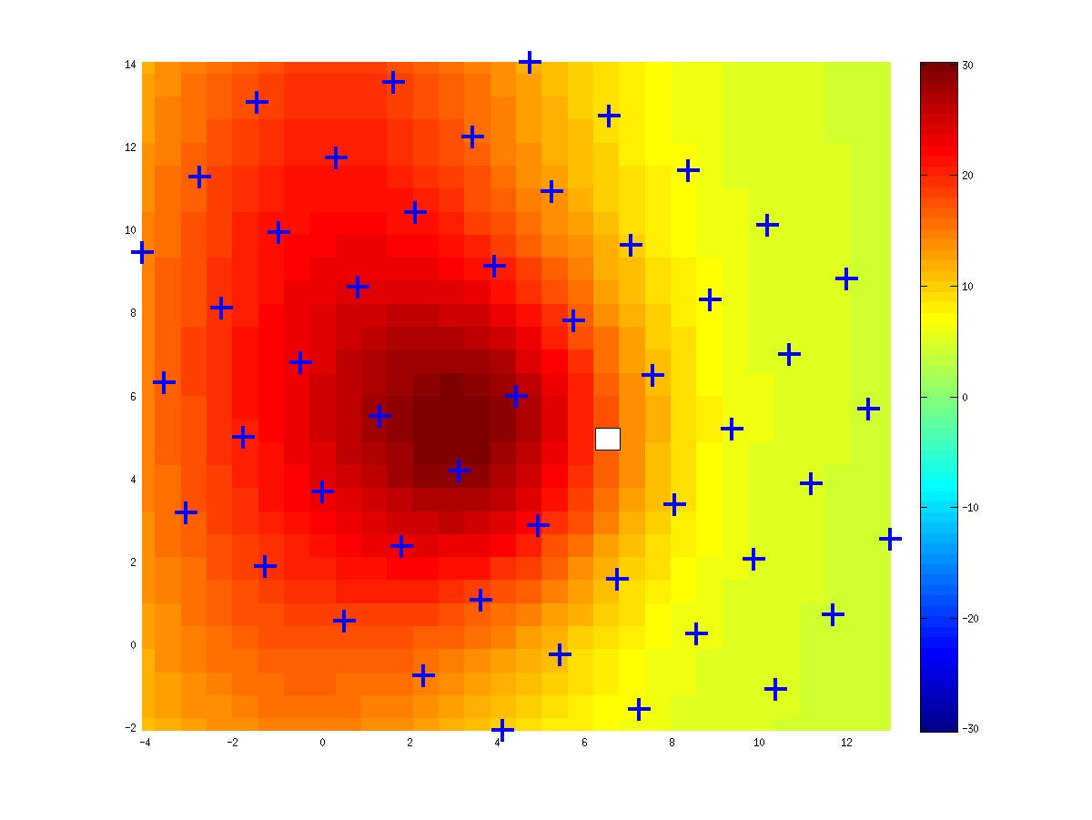
This model can account for the modifications of the receptive field shape we mentioned previously namely the increase of the response of the neuron on the side of the RF where spatial attention is focused and a decrease of the response on the other flank. For example, suppose we have an unmodulated receptive field centered at (0,0), the anti-preferred stimuli being at (2, 2) and (2, -2). We consider three situations. In the unmodulated situation, or attend-away, attention is supposed to be sufficiently far to have no influence on the receptive field. In the attend-s1 or attend-s2 conditions, attention is supposed to be on respectively the anti-preferred stimulus S1 or S2. With some arbitrary values for the parameters, we plot below the responses and difference maps in these different conditions.
| Attend away | Attend s1 | Attend s2 |
|---|---|---|
 |
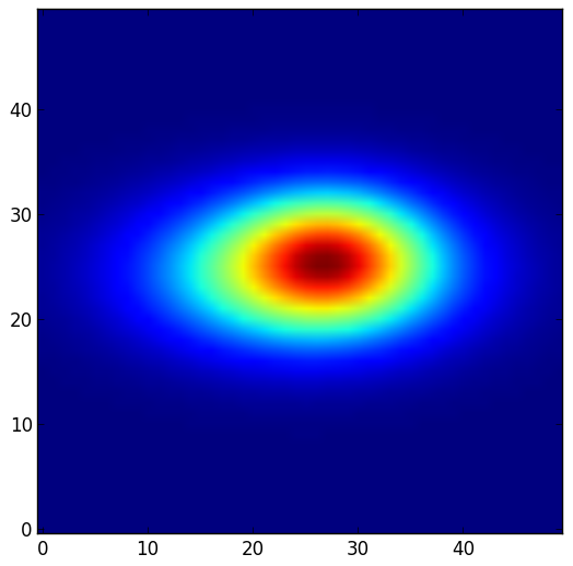 |
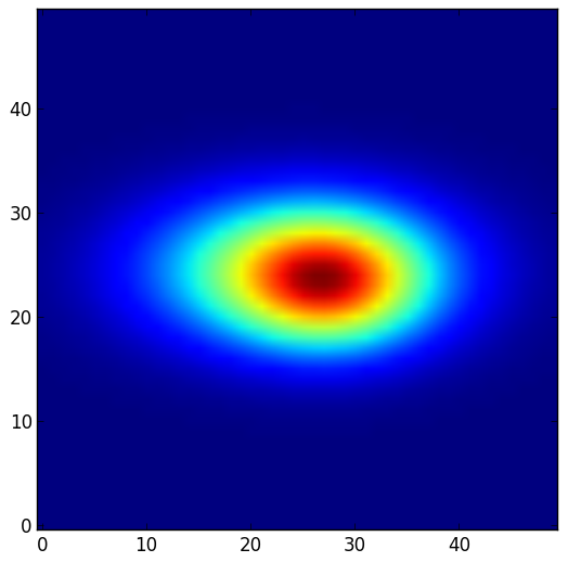 |
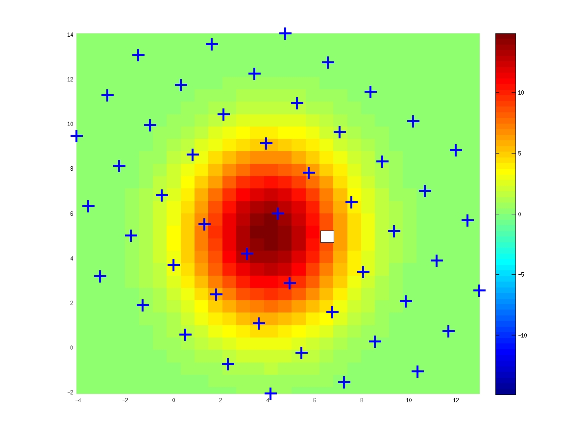
Now the difference maps:
| Difference attend s1 - attend away | Difference attend s2 - attend away | Difference attend s1 - attend s2 |
|---|---|---|
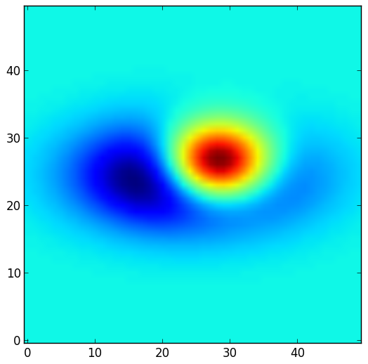 |
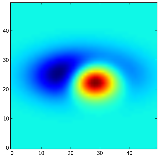 |
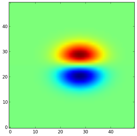 |
We see that the model can potentially replicate the increase of the RF on the attentional side and the decresase of the RF on the opposite flank which explains the RF shape modifications (shift and shrinkage).
Fitting the model
Let us consider again the sample RF we plotted at the very beginning and which was fitted with splines. Fitting the model to the data means finding 11 parameters. There are 7 parameters defining the unmodulated receptive field (be carefull, this is different from the attend away condition where S1 and S2 influences the unmodulated RF) which are the center (2), the variances (2), the orientation, peak and baseline (3). The anti-preferred stimuli introduce two additional parameters (A1, A2) and the attentional signal 2 more (Ap and Sp). The anti-preferred stimuli are placed at the same eccentricity and therefore we assume that the attentional signal has the same shape wheter the monkey attended to S1 or S2 (in general, one might assume that the shape of the attentional signal varies with the eccentricity of attention). However, the two inhibitory influences A1 and A2 must be kept seperated as the anti-preferred stimuli are not necessarily symmetrically positioned within the receptive field of the neuron. The recordings do not contain the unmodulated situation and we must therefore fit all the three conditions simultaneously.